UMAP

The UMAP dimensionality reduction tool offers a workflow for dimensionality reduction and clustering that is particularly useful for high dimensional data, such as hyperspectral images. The tool uses UMAP (Uniform Manifold Approximation and Projection) to reduce the dimensionality of the data, followed by HDBSCAN (Heirarchical Density Based Spatial Clustering of Applications with Noise).

Selecting data

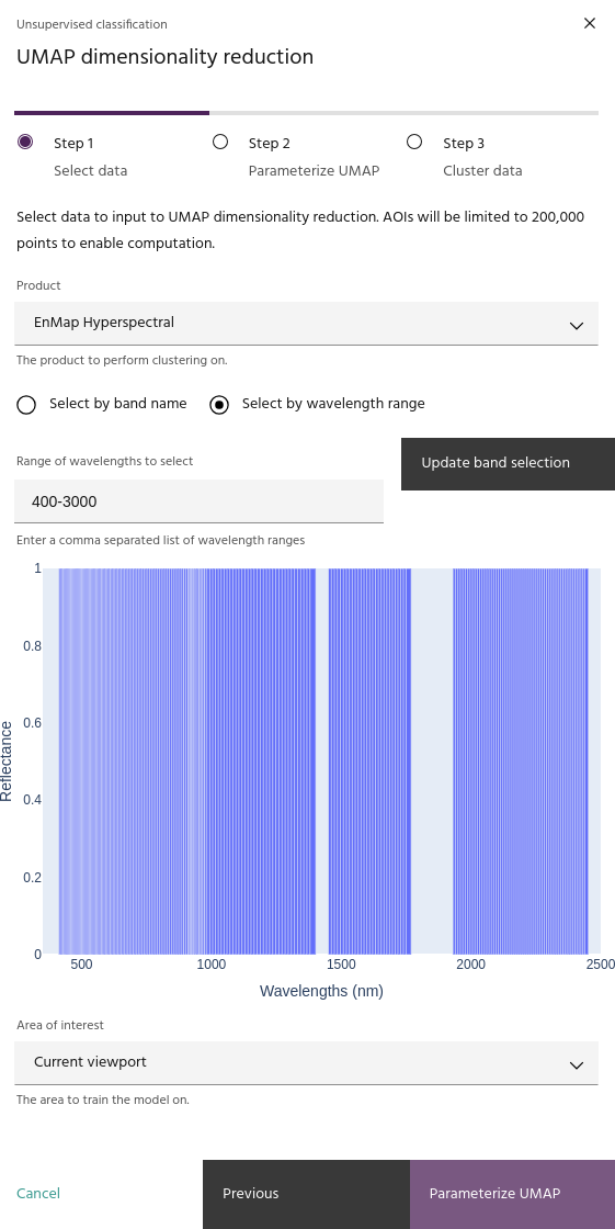
The UMAP dialog is broken into three steps. The first step allows you to select the product, bands and AOI for analysis. When you have selected the data you want to analyze, click Parameterize UMAP to move to the next step.

Parameterize UMAP

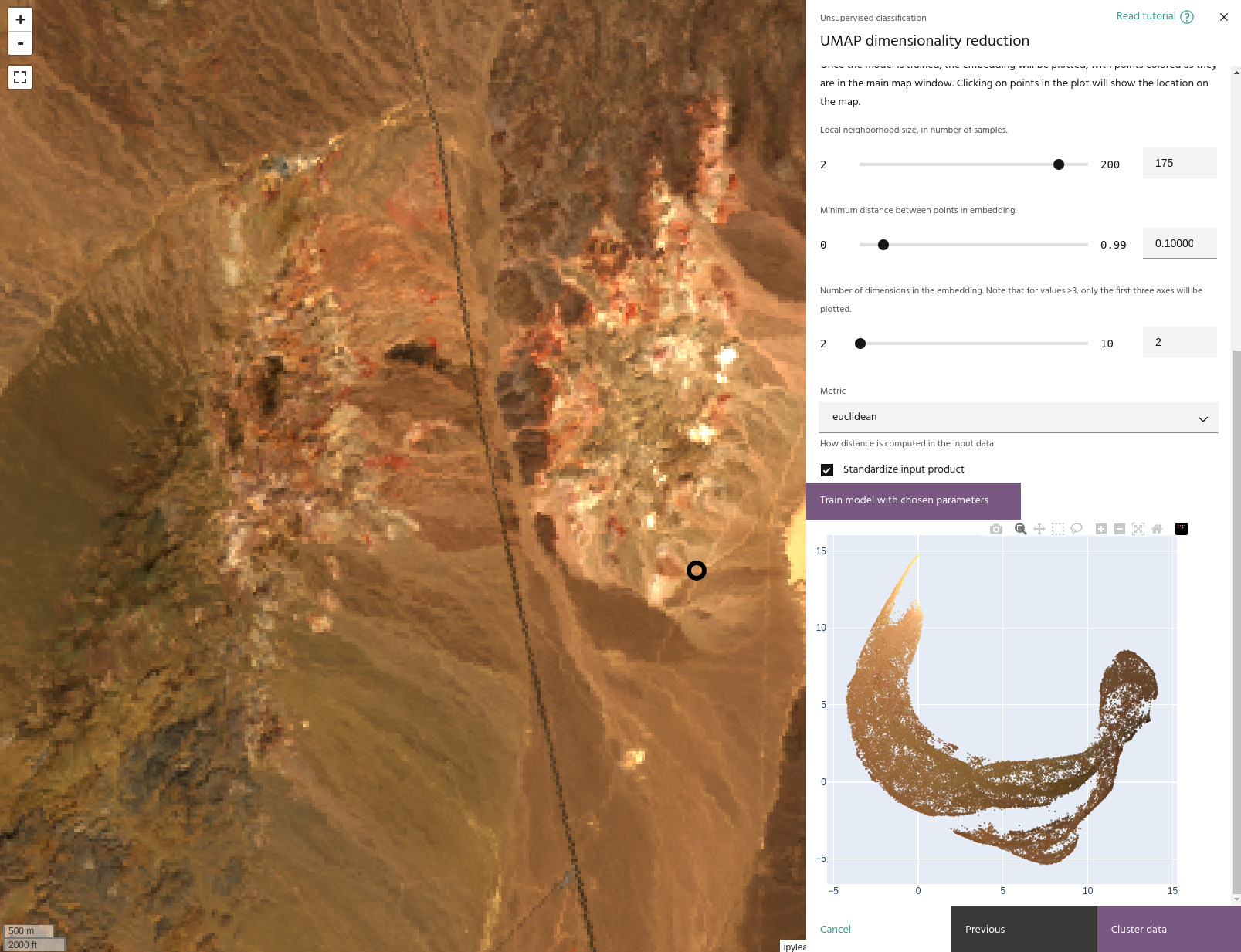
UMAP works by computing a manifold of the input data and projecting that manifold to a lower dimensional space. Parameterizing UMAP, therefore, involves determining how that manifold is built (the neighborhood size and distance metric used), how many dimensions to use in the projection, and how clustered the low dimensional projection is. The second step of the dialog allows manipulation of these parameters and provides a plot of the embedding for analysis. When you have set parameters to your satisfaction, click Train model with chosen parameters to train the model and generate a plot of the embedding, and when you are satisfied with your model click Cluster data to move to the clustering step.

Local neighborhood size

The number of points that UMAP will use when building the data manifold. This parameter allows a balance between local and global structure of the data in the embedding - low values will focus on local structure, and large values will focus on global structure.

Minimum distance

The minimum distance between points in the final embedding. Lower values will create a clumpier embedding, while larger values will spread points farther apart.

Number of dimensions

Number of dimensions for the embedding. Unlike simpler embedding algorithms such as T-SNE, UMAP can successfully embed into more than three dimensions.

Metric

The metric for computing distances in the input data. Available metrics are:

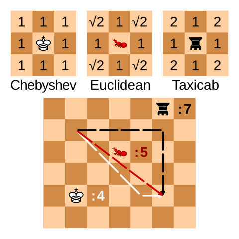
• Euclidean: Simple Euclidean distance between points.
• Manhattan: Manhattan, or "Taxi cab" distance, measures the sum of the distance along each axis.
• Chebyshev: The Chebyshev metric defines the distance between points as the greatest of their differences along any axis.
• Cosine: Cosine distance is the cosine of the angle between the vectors.
• Correlation: Correlation distance between the vectors, measuring the dependence between them.

Embeddings plot

After training a model, the embedding will be plotted on either a 2D or 3D scatterplot, depending on the choice of dimension. Points on the plot will be colored the same as they are on the map, and clicking on plotted point will show the location on the map in a vector layer called selected points.

Cluster data

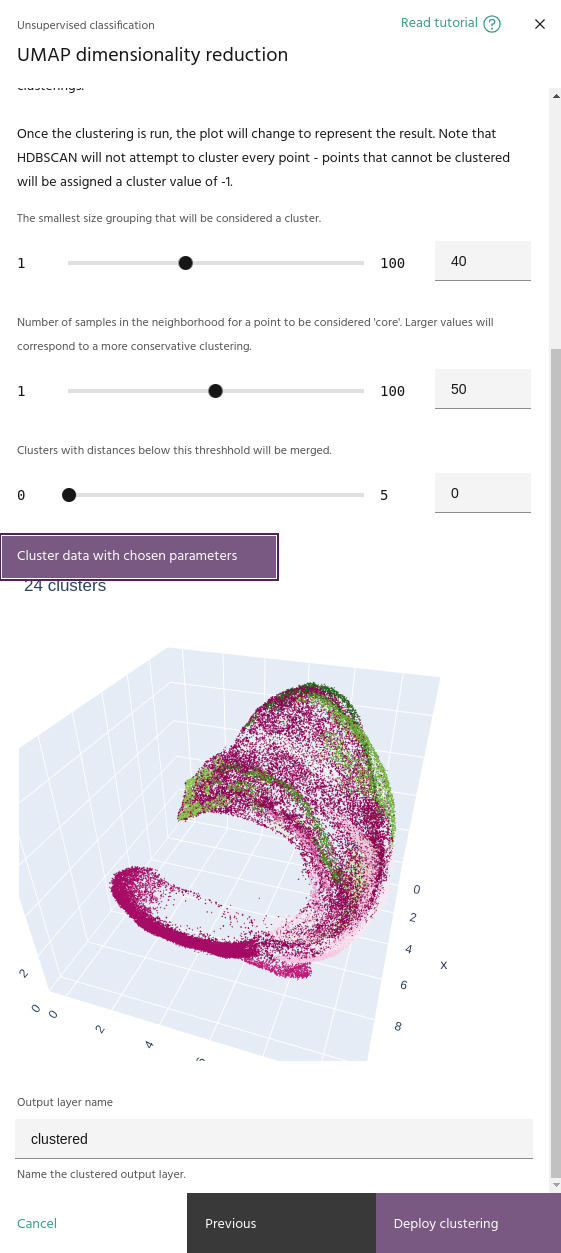
Once the low dimensional manifold is built, the UMAP tool uses HDBSCAN to cluster the data in an unsupervised manner. HDBSCAN is a better clustering algorithm than k-means for the unique shapes that are generated with UMAP, as it can find clusters with varied shapes, whereas k-means builds clusters as balls. Use the Cluster data with chosen parameters button to run the clustering on your embedded data.

Minimum cluster size

The smallest number of points that can be considered a cluster. Lower values tend to create more clusters.

Minimum number of samples

The minimum number of samples in the neighborhood of a point for it to be considered a "core" sample, and therefore considered for clustering instead of noise.

Cluster selection epsilon

This parameter merges clusters that are closer than this value. This will help if your clustering contains a large number of small, nearby clusters.

Deploy clustering

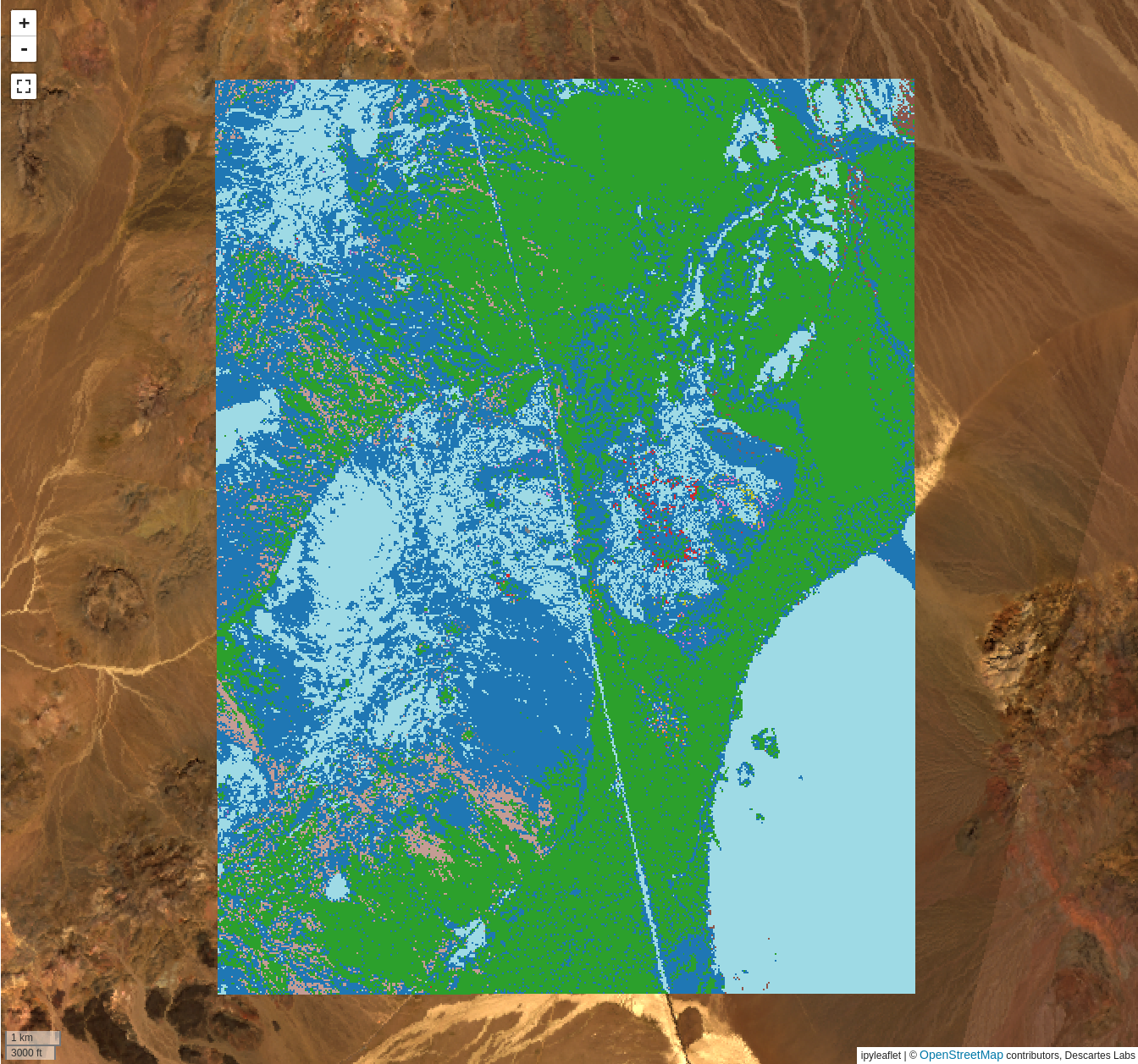
When you are happy with the clustering parameters, click the Deploy clustering. This will deploy a Compute function that will apply the UMAP and HDBSCAN models over your chosen AOI, and add the result to the map.